Creative morphometrics

Using R and python for colorful research of biological shape

Python Forcing Monsters` Shape

Continuing on one of the previous posts about data generation in python, next natural step in the analytic procedure is the Procrustes superimposition. Since this procedure enables direct analyses of configurations` shape, and all subsequent explorative visualizations, it must be employed first. This post concerns with the basic superimposition procedure, involving only two landmark configurations, i.e. two generated monsters. One monster will be used as a reference and one as a target, which should undergo superimposition. First steps in data genration are the same as before, with the exception of polarRotator function that can take any numpy array and reorder it according to polar rotation angle. This is very useful since generated landmarks are not ordered properly and do not “feel natural” in plots and analyses.

Library import, data generation and some functions
1
2
3
4
5
6
7
8
9
10
11
12
13
14
15
16
17
18
19
20
21
22
23
24
25
26
27
28
import numpy as np
import pandas as pd
import matplotlib.pyplot as plt

def centsize(M):   #centroid size of any configuration matrix
  p = M.shape[0]
  csize = np.sqrt(np.sum(M.var(0))*(p-1))
  return csize

def polarRotator(M):   #polar rotation for natural ordering of landmarks
  x = np.array(M[:,0])
  y = np.array(M[:,1])
  points = np.array((x,y)).T
  cent = (np.sum(x)/len(M), np.sum(y)/len(M))
  angle = np.arctan2(points[:,1]-cent[1],points[:,0]-cent[0])
  points = pd.DataFrame(points, columns = ['x','y'])
  angle = pd.Series(angle)
  points['angle'] = angle
  points = points.sort('angle')
  rotatedMat = np.array(points[['x','y']])
  return rotatedMat

coordstest = np.vstack([np.random.uniform(175, 220, 10), np.random.uniform(175, 220, 10)]).T
monster1 = np.vstack([np.random.multivariate_normal(coordstest[i,:], [[3,0],[0,3]], 1) for i in range(10)])
monster2 = np.vstack([np.random.multivariate_normal(coordstest[i,:], [[3,0],[0,3]], 1) for i in range(10)])

monster1 = polarRotator(monster1)
monster2 = polarRotator(monster2)

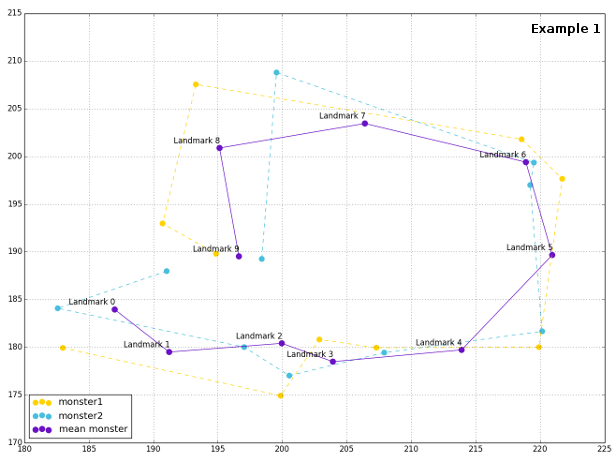
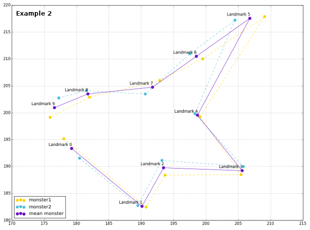
The plot of configurations reveals their spatial relationship, as well as the general mean shape. This time, since landmarks are ordered properly, one line would be enough for representing mean shapes, and shapes of respective configurations.

Plotting the original monsters
1
2
3
4
5
6
7
8
9
10
11
12
13
14
15
plt.scatter(monster1[:,0], monster1[:,1], s = 80, c = "#FFD200", edgecolors = 'none', label = "monster1")
plt.plot(monster1[:,0], monster1[:,1], '--', color = "#FFD200")
plt.scatter(monster2[:,0], monster2[:,1], s = 80, c = "#47BFDD", edgecolors = 'none', label = "monster2")
plt.plot(monster2[:,0], monster2[:,1], '--', color = "#47BFDD")

meanMon = (monster1 + monster2) / 2 #calculate mean shape
plt.scatter(meanMon[:,0], meanMon[:,1], s = 90, c = "#6a12c4", edgecolors = 'none', label = "mean monster")
plt.plot(meanMon[:,0], meanMon[:,1], '-', color = "#6a12c4")

labels = ['Landmark {0}'.format(i) for i in range(10)]
for label, x, y in zip(labels, meanMon[:,0], meanMon[:,1]): #annotate mean landmarks by numbers
  plt.annotate(label, xy = (x, y+0.3), ha = 'right', va = 'bottom')

plt.grid()
plt.legend(loc = "lower left")

Procrustes superimposition revolves around three features of shape extraction, that is invariance of landmark configurations to position, scale and rotation. There are a number of excelent textbooks about the mathematics and logic, as well as procedures for Procrustes superimposition (Bookstein, 19911, Dryden and Mardia, 19982, Zelditch et al., 20123), but for this post direct inspiration was Morphometrics in R (Claude, 2008), especially with the basic procedure presented in the following function definition.

Partial Procrustes superimposition of two configurations
1
2
3
4
5
6
7
8
9
10
11
12
13
14
15
16
17
18
19
20
21
22
23
def pProc(mat1, mat2):
  k = mat1.shape[1]-1
  m = mat1.shape[0]
  sscaledMat1 = mat1 / centsize(mat1) #scaling and centering
  sscaledMat2 = mat2 / centsize(mat2)
  z1 = sscaledMat1 - [sscaledMat1[:,0].mean(), sscaledMat1[:,1].mean()]
  z2 = sscaledMat2 - [sscaledMat2[:,0].mean(), sscaledMat2[:,1].mean()]
  tempSv = np.dot(np.transpose(z2), z1) #rotation
  svdMat = np.linalg.svd(tempSv)
  U = svdMat[0]
  V = svdMat[2]
  Ds = svdMat[1]
  tempSig = np.linalg.det(np.dot(np.transpose(z1), z2))
  sig = np.sign(tempSig)
  Ds[k] = sig * np.absolute(Ds[k])
  U[:,k] = sig * U[:,k]
  Gam = np.dot(V, np.transpose(U))
  beta = np.sum(Ds)
  pmat1 = np.dot(z1, Gam)
  pmat2 = z2
  tempRot = vstack((pmat1, pmat2))
  rotatedMat = pd.DataFrame(tempRot, columns = ['x','y'])
  return rotatedMat

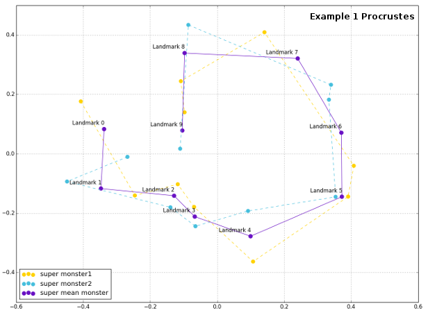
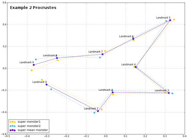
Plot of the superimposed configurations reveals that the Procrustes python was really able to force monsters` shape be more similar, removing the effects of orientation, size and rotation.

Plot of the superimposed configurations
1
2
3
4
5
6
7
8
9
10
11
12
13
14
15
16
17
18
19
rotatedMon = pProc(monster1, monster2)
rotatedMon1 = np.array(rotatedMon[:10])
rotatedMon2 = np.array(rotatedMon[10:20])

plt.scatter(rotatedMon1[:,0], rotatedMon1[:,1], s = 80, c = "#FFD200", edgecolors = 'none', label = "super monster1")
plt.plot(rotatedMon1[:,0], rotatedMon1[:,1], '--', color = "#FFD200")
plt.scatter(rotatedMon2[:,0], rotatedMon2[:,1], s = 80, c = "#47BFDD", edgecolors = 'none', label = "super monster2")
plt.plot(rotatedMon2[:,0], rotatedMon2[:,1], '--', color = "#47BFDD")

meanRotMon = (rotatedMon1 + rotatedMon2) / 2
plt.scatter(meanRotMon[:,0], meanRotMon[:,1], s = 90, c = "#6a12c4", edgecolors = 'none', label = "super mean monster")
plt.plot(meanRotMon[:,0], meanRotMon[:,1], '-', color = "#6a12c4")

labelsRot = ['Landmark {0}'.format(i) for i in range(10)]
for label, x, y in zip(labelsRot, meanRotMon[:,0], meanRotMon[:,1]): #annotate mean landmarks by numbers
  plt.annotate(label, xy = (x, y+0.01), ha = 'right', va = 'bottom')

plt.grid()
plt.legend(loc = "lower left")

Following posts should continue on this one and describe how the partial Procrustes superimposition for multilple configurations can be performed with fabulous sientific python.


  1. Bookstein, F.L. 1991. Morphometric tools for landmark data: Geometry and Biology. Cambridge University press, Cambridge, UK.

  2. Dryden, I.E. and K.V. Mardia. 1998. Statistical shape analysis. Wiley, Chichester, UK.

  3. Zelditch, M.L., Swidersk, D.L. and H.D. Sheets. 2012. Geometric morphometrics for biologists: A primer. Second edition, Elsevier.