With the ongoing expand of the available geospatial databases in raster format (GeoTiff) it is getting easier to analyse the relationship between any complex morphology, captured in landmark data, and i.e. climate or precipitation data with the help of partial least squares (PLS). R has a wonderful raser, sp and gdal packages that facilitate the extraction of the geospatial data from GeoTiff raster grids. In this post the geoTiff used will be from the WorldClim website, and the climate data for European square 16, where some of my real samples originate from. In order to get this data you can follow the downloads section of the WorldClim website and choose download data by tile, 30 arc-seconds resolution. When a map opens the dataset for this post would be under the map, when clicked on the square zone 16 and finally download the Mean Temperature. This is a .zip file with twelve GeoTiffs, one for each month. Unpack the files in a pre-destined directory, and declare this a working directory in the R session.

1
2
3
4
5
6
7
8
9
10
11
12
13
14
15
16
17

setwd("~/tmean") #this is the folder with all the GeoTiffs
library(raster)
library(sp)
library(rgdal)
meanJan <- raster("tmean1_16.tif") #mean temp for January etc.
meanFeb <- raster("tmean2_16.tif")
meanMar <- raster("tmean3_16.tif")
meanApr <- raster("tmean4_16.tif")
meanMaj <- raster("tmean5_16.tif")
meanJun <- raster("tmean6_16.tif")
meanJul <- raster("tmean7_16.tif")
meanAvg <- raster("tmean8_16.tif")
meanSep <- raster("tmean9_16.tif")
meanOkt <- raster("tmean10_16.tif")
meanNov <- raster("tmean11_16.tif")
meanDec <- raster("tmean12_16.tif")
plot(meanJan) #will simply get the basic R plot of a GeoTiff raster

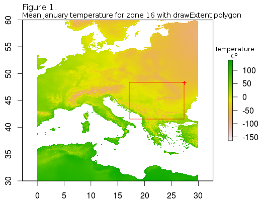
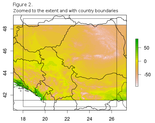
After reading in the basic data, raster package offers several formats in which to keep the data, besides the basic raster. The most useful one is a raster stack which really is just the piled-up rasters that can be manipulated together. Also one useful visual help is the addition of the country boundaries followed by zooming in to the extent of the country or region where the samples originate from. Country boundaries .shp files is freely avalilable from thematicmapping. When downloaded they should be in the same directory as the GeoTiffs.

1
2
3
4
5
6
7
8
9
10

mtStack <- stack(meanJan, meanFeb, meanMar, meanApr, meanMaj, meanJun, meanJul, meanAvg, meanSep, meanOkt, meanNov, meanDec)
bounds <- readOGR(dsn=getwd(), layer= "TM_WORLD_BORDERS-0.3") #import borders
plot(meanJan) #plot the raster file for any month
extentR <- drawExtent()
#drawExtent enters the interactive mode where you can draw the polygon for zooming based on two points, top right and lower left
#values in extentR are coordinates in WGS84 datum and expressed as longitude data
plot(zoom(bounds, extentR), add = TRUE)
#unfortunately this does not work well since it will plot the bounds in the zoom extent
#and if the both raster and bounds are needed then it might be ok to overlap them in GIMP
plot(zoom(meanJan, extentR), add = TRUE)

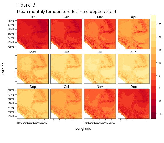
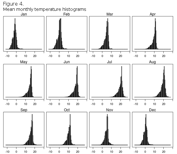
Before final extraction of the climate data it can be useful to plot each month`s mean temperature for the selected extent of the rasater. This can be easily achieved by using the rasterVis package levelplot and the extentR variable, which can be used to cut through all raster layers in the stack.

1
2
3
4
5
6

library(rasterVis)
cutStack <- (crop(mtStack, extentR))/10
#division by 10 is needed since the temperature data in this GeoTiff is x10 for saving memory-important
names(cutStack) <- month.abb
levelplot(cutStack) #may take long time to plot
histogram(cutStack)

Slightly more efficient than the drawExtent is the spatialPolygons function from the sp package that will be used for definition of the real sampling localities, by simply drawing boundaries of the localities by hand or using the known positional data. It is best if approximate latitude/longitude coordinates are known in advance so that the defining polygon can be drawn connecting several corners-points, that form the broader sampling area border. If coordinates are not known in advance then the drawExtent should be used first for finding the latitude/longitude of the spatial polygon points, and then making the SpatialPolygon object out of them, as described next.

1
2
3
4
5

taraCoord <- rbind(c(19.241867, 44.012571), c(19.351730, 43.976511), c(19.518585, 43.923121), c(19.435501, 43.894924), c(19.317398, 43.896903), c(19.261780, 43.955259), c(19.241867, 44.012571))
R1Coord <- rbind(c(24.656067, 45.627484), c(25.252075, 45.575600), c(25.628357, 45.525592), c(25.488281, 45.3000007), c(25.046082, 45.381080), c(24.672546, 45.539060), c(24.656067, 45.627484))
#these objects are matrices with two columns, one for latitude of a polygon corner and the other the longitude
polyTara <- SpatialPolygons(list(Polygons(list(Polygon(taraCoord)), 1))) #declare object type
polyR1 <- SpatialPolygons(list(Polygons(list(Polygon(R1Coord)), 1)))

After all spatial polygons are defined, final step involves the extraction of the mean temperature values from the points encircled by the polygon in question, for all months. Since GeoTiffs are raster formats, they are carrying the information on the temperature in the points of the bitmap grid, so if the polygon is too small, small will be the number of the grid-points inside, maybe smaller than the number of individuals. To avoid this make sampling area broader, and in this case polyTara has some 220 individual grid points inside, which means 220 values for the mean temperature in the area. If we have i.e. ten individuals per population it is necessery to have also 10 mean temperature values, so that both blocks in subsequent PLS would have same dimensionality. R`s basic sample function can be used to extract random values from the i.e. 220 points within the population (Tara and R1) polygons. This simulates random sampling of individuals from the sampling locality and after that any analysis can be done, from linear models to PLS, which will be shown in future posts.

1
2
3
4
5
6
7
8
9
10
11
12
13
14

matTaraMean <- extract(cutStack, polyTara)[[1]]
matR1Mean <- extract(cutStack, polyR1)[[1]]
plot(cutStack$Jan)
plot(polyTara, add = TRUE)
plot(polyR1, add = TRUE)
n <- dim(matTaraMean)[1] #for sampling convenience
m <- dim(matR1Mean)[1]
taraMat <- matTaraMean[sample(n, 10),] #this is the final extracted data
R1Mat <- matR1Mean[sample(m, 10),]
library(ggplot2)
library(reshape2)
plotter <- data.frame(rbind(taraMat, R1Mat), loc = c(rep("Ta",10), rep("R1", 10))) #for ggplot2
forplo <- melt(plotter)
m <- ggplot(forplo, aes(x = value, fill = loc)) + geom_histogram() + facet_grid(variable~.)

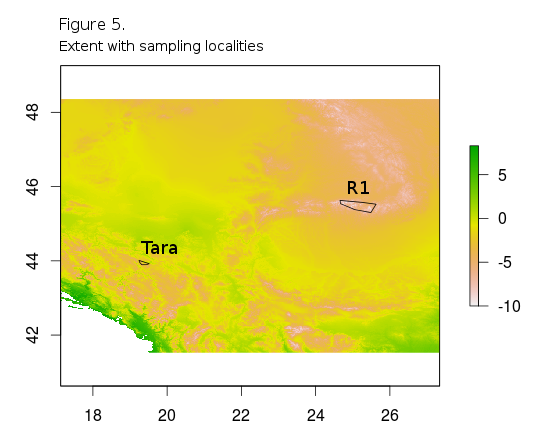
Figure 5. shows the locations of tara and R1 spatial polygons within the zoomed extent of the zone 16, while in Figure 6. barplots are shown for 10 random points for all months, and for both localities, for comparison.

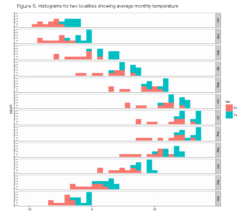
It is obvious that the Tara locality has higer mean monthly temperature, on average for every month, and also it has less temperature variaton than R1.