Continuing on the previous post, procedures presented here show the comparison between the usual assesment of modularity in the collection of landmarks (same dataset as before) and the depiction of modular structure through graph theory. Usually, modularity in the mammalian cranium is determined a-priori, according to some of the established hypotheses about the developmental origin of cranial elements. One of the most prevalent hypotheses is the two-module organization, one module comprising of elements originating mainly from the neural crest embryonic tissue (anterior cranium) and one comprising of elements with somitomeric origin (posterior cranium). Following code shows the test of this specific hypothesis using geomorph package functions, and additional usage of deldir for visualization of modularity hypotheses.

1
2
3
4
5
6
7
8
9
10
11
12
13
14
15
16
17
18
19

library(geomorph)
library(deldir)
library(ggplot2)
load("capSample.RData")
theme_set(theme_bw())

capGPA <- gpagen(capSample)
capCoords <- capGPA$coords
mshapeCap <- mshape(capCoords) #mean shape is useful for plotting 

#vector depicting the division of landmarks according to modularity 
modularity1.gps <- c("A","A","A","A","A","A","A","A","B","B","A","B","B","B","B","B")
#test for modularity based on the RV coefficient
modularity1 <- compare.modular.partitions(capCoords, landgroups = modularity1.gps)
#plot of landmark membership to a-priori modules
deldir(mshapeCap[,1], mshapeCap[,2], plotit = TRUE, wlines = "triang", xlim = c(-0.2,0.55))
points(mshapeCap[c(1:8,11),1], mshapeCap[c(1:8,11),2], col = "#FF8740", pch = 19, cex = 1.2)
points(mshapeCap[c(9,10,12:16),1], mshapeCap[c(9,10,12:16),2], col = "#61B4CF", pch = 19, cex = 1.2)
legend(0.2,0.4, legend = c("neural crest", "somitomere"), fill = colormap)

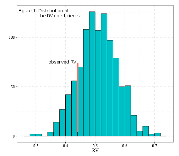
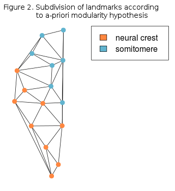
Figure 1 shows the theoretical distribution of the RV coefficients, calculated for all posible two-module subdivisions of landmarks, as well as the observed RV value from the hypothesis depicted in Figure 2. Since the observed value is lower than most of the hypothetic values, then it could be said that this modularity hypothesis stands.

The idea for using graph theory representation and analysis of modularity is based on correlation matrix, same one from the previous post. Correlation matrix was obtained through Delaunay triangulation and every vertex (node) in the graph actually represents the 1/3 of the total area of all Delaunay triangles emanating from the corresponding landmark.

1
2
3
4
5

cicoCap <- t(apply(capCoords, 3, function(A) deldir(A[,1],A[,2])$summary[,4]))
cicoCap <- data.frame(cicoCap)
names(cicoCap) <- paste("lm", c(1:16), sep = "")
capCor <- abs(cor(cicoCap)) #correlation matrix
diag(capCor) <- 0 #diagonals must be set to zero

Graph based on the correlation matrix can be created and manipulated with the wonderful igraph package. Vertices of this graph will be abovementioned areas, while the edges will represent correlation (edge weights) between areas around each landmark. According to weights, edges can be colored and the strength of thier lines increased, so that the most correlated landmarks wolud be more obvious.

1
2
3
4
5

graph <- graph.adjacency(capCor, weighted=TRUE, mode="upper")
E(graph)[ weight > 0.5 ]$color <- "#A63E00"
E(graph)[ weight > 0.5 ]$width <- 3.6
E(graph)[ weight > -0.5 & weight < 0.5 ]$color <- "#D6EBFF"
E(graph)[ weight > -0.5 & weight < 0.5 ]$width <- 1.2

Modularity, or community structure in the graph theory represents the degree of compartmentalization in the graph structure, based on the spatial relationship or the weights of graph edges. Although, a-priori subdivision of graph vertices is possible, and the evaluation of such graph community can be easily done, the advantage of graph theory for modularity is the availability of algorithms for searching the community structure, so it can derive subdivsion a-posteriori, that can be compared to the hypothesis from Figure 1.

1
2
3
4
5
6
7
8
9
10
11

gsc <- leading.eigenvector.community(graph, weights = E(graph)$weights)
modularity(graph, membership(gsc))
colormap <- c("#FF8740", "#61B4CF")
V(graph)$color <- colormap[gsc$membership] #color graph vertices according to community

#graph layout will be circular since values for the edges range from 0.2 to 0.9, 
#and they all form similar attractive force between the vertices.
graph$layout <- layout.fruchterman.reingold #really no effect on the shape of this graph

plot(graph, vertex.size = 20, vertex.shape = "circle")
legend(0.8,1.4, legend = c("neural crest", "somitomere"), fill = colormap)

Leading eigenvector community algorithm tries to find community structure in the graph by calculating the eigenvector of the modularity matrix for the largest positive eigenvalue and then separating vertices into two communities based on the sign of the corresponding element in the eigenvector (Newman, 2006¹). This method was preffered over many others because it is closer to usual multivariate methods, such as PCA, that are commonly used to depict variability patterns.

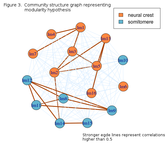
Graph community strucure depicts modularity in the landmark configurations accurately, with the exception of lm16, that is positioned on the posterior basicranium. Higher correlations are, on average, present within modules while between modules, only one connection is higher than 0.5, that between lm2 and lm14. Since these landmarks lay on the opposite sides of the cranium, they may encompass the variability in total anterior-posterior length. i.e. cranial size.