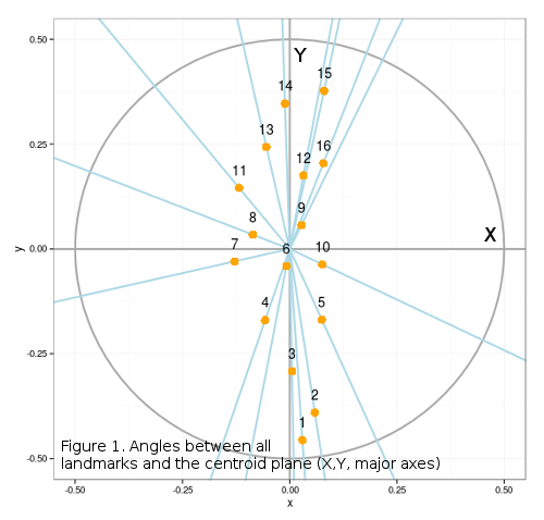
Angles were important for some of the most interesting research in morphometrics. The approach of Rao and Suryawanshi, 1998¹. introduced the angles within the landmark triangulation grids as an alternative to Procrustes superimposition for extracting shape data. This post does not perform the procedures described by Rao (which are ported to R in “Geometric morphometrics in R” by J.Claude, 2008), but instead aims at extracting angle data, from configurations of landmarks, after Procrustes superimposition. The code presented here is motivated by the polarRotator function from some of the previous pyhton-related posts, and it presents landmark data as polar angles. These angles represent the angular deviation of each landmark from the centroid of the respective configuration (Figure 1), so that the variability in their position with respect to xy centroid coordinates, may represent their shape differences. Since superimposition procedure sets all configurations centroids to the origin, they are all 0,0. Dataset used is the same as for the triangulation post.

1
2
3
4
5
6
7
8
9
10
11
12
13
14
15
16
17
18
19
20
21
22
23
24
25
26
27
28
29
30
31
32
33

library(geomorph)
library(ggplot2)
library(reshape2)
library(plyr)
theme_set(theme_bw())

load("capSample.RData")

capGPA <- gpagen(capSample)
capCoords <- capGPA$coords
mshapeCap <- mshape(capCoords) #mean configuration is great for illustrations
capCentro <- capGPA$Csize

circleFun <- function(center = c(0,0), npoints = 100) #drawing an enlosing circle set at the origin (0,0)
{
  r = 0.5
  tt <- seq(0,2*pi,length.out = npoints)
  xx <- center[1] + r * cos(tt)
  yy <- center[2] + r * sin(tt)
  return(data.frame(x = xx, y = yy))
}

enclosing <- circleFun(npoints = 100) #it should be centered at zero and have diameter 0.5
ggCirc <- ggplot(enclosing, aes(x=x,y=y)) + geom_path(size = 1, color = "darkgrey", linetype = 1)
ggCirc <- ggCirc + geom_hline(size = 1, color = "darkgrey", linetype = 1) + geom_vline(size = 1, color = "darkgrey", linetype = 1)

linesAng <- data.frame(x1 = c(0, 0, 0, 0), y1 = c(0, 0, 0, 0), x2 = mshapeCap[,1], y2 = mshapeCap[,2]) #point coordinates
linesAng <- data.frame(linesAng, x3 = linesAng$x2 * 20, y3 = linesAng$y2 *20) #so that the lines would extend through landmarks

ggCirc <- ggCirc + geom_segment(data = linesAng, aes(x = x1, y = y1, xend = x3, yend = y3), colour = "lightblue", size = 1)
ggCirc <- ggCirc + geom_point(size = 4.2, color = "orange", data = data.frame(mshapeCap), aes(x=X1, y = X2))
ggCirc <- ggCirc + geom_text(data = data.frame(mshapeCap), aes(x=X1, y = X2, label = c(1:16)), vjust = -1.2)
ggCirc <- ggCirc + coord_cartesian(xlim= c(-0.55, 0.55), ylim= c(-0.55, 0.55))

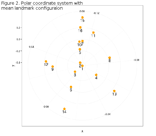
ggplot2 has one great geom, polar_angle() that will transform any shape, from Cartesian to polar coordinates. Unfortunately it does not give polar angles as well, but the plot is informative (Figure 2), since landmarks are ordered according to their angular deviation from 0, i.e. the X and Y axes defining the 0.5 centroid-centered ellipse.

1
2
3

ggPolar <- ggplot(data.frame(mshapeCap), aes(x=X1, y=X2)) + geom_point(size = 4.2, color = "orange")
ggPolar <- ggPolar + geom_text(aes(label = c(1:16)), vjust = 1.5)
ggPolar <- ggPolar + coord_polar(start = 0) + xlab("x") + ylab("y")

Polar angles can be calculated by using the atan2 (arctangent) function, which takes two parameters, x and y and gives one point estimate of the polar angle in radians. This number is really the angle between the positive x-axis of a plane (X from Figure 1) and the point given by its xy coordinates. Since after superimposition the x-axis lies at zero for all landmark configurations, it would be sufficent to use only xy coodinates of landmarks, since centroids are also at 0.

1
2
3
4
5
6
7
8
9
10
11
12
13
14
15
16
17
18
19
20
21
22
23
24
25
26

polarAngler <- function(A) #function to calculate polar angles from the array
{
  siz <- dim(A)[3]
  len <- dim(A)[1]
  polarAngles <- vector("list", siz)
  for (i in 1:siz)
  {
    temp <- atan2(A[,2,i], A[,1,i])
    polarAngles[[i]] <- temp
  }
  polarAngles <- array(unlist(polarAngles), dim = c(len,1,siz))
  return(polarAngles)
}

library(circular)
library(colortools)

pAngles <- polarAngler(capCoords) #angles for all configurations
mAngles <- apply(pAngles, 1, mean) #mean angles for each landmark
col1 <- pals("fish") #paletes from colortools
col2 <- pals("ocean")
col3 <- pals("mystery")
colorPoint <- c(col1, col2, col3, "#9A76F5") #16 colors for landmarks in whell

plot.circular(circular(t(mAngles), type = "angles"), sep = 0.0003, col = colorPoint, cex = 1.5)
legend(0.3,0.6, legend = 1:16, fill = colorPoint, cex = 0.7)

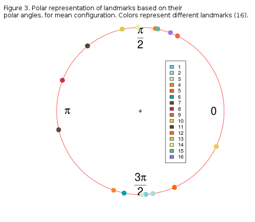
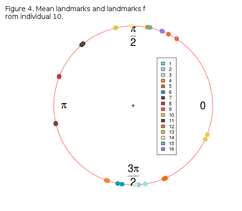
Figure 3 shows the distribution of landmarks from along a circular path (0, π). It is obvious that landmarks form two distinct groups, one above, and one below the x-axis, with the exception of landmarks 7, 8 and 10 which are the most parallel to the x-axis. The proportion of the overall shape variability left in these angles must be thouroghly checked, but it is not easy, since angle-data can not be analysed by conventional statistics, but by circular or compositional methods. R provides some libraries for this, circular and CircStats which are both derived from the book of Jammalamadaka and Sengupta, “Topics in circular Statistics” from 2001. If one more individual is added to the circle-plot (Figure 3) it can be can visually inspected how much its coordinates (landmark polar angles) deviate from the sample mean (Figure 4).

1
2
3

ce <- circular(rbind(t(mAngles), pAngles[,,10])) #deviation of individual 10 from the mean
plot.circular(ce, sep = 0.0003, col = colorPoint, cex = 1.5)
legend(0.3,0.6, legend = 1:16, fill = colorPoint, cex = 0.7)

Some variablity is present around landmarks 10, 6 and 5, while others are nearly or completely overlapping. The variability may not be large, but it will be checked in future posts, as well as possible PCA with the angular data.