Quantification of biological shape often relies on manual extraction of information from a set of digital images or 3D models, like manual landmark placement or outlining the object of interest by hand. With computer vision approach and, especially, with the help of the openCV library, a set of image manipulation tecniques as well as automated feature extractions are facilitated to a large extent. Since there are excellent python bindings for this library it is easy to test ideas for image analysis and object extraction in the context of geometric morphometrics.

This post will serve as a general introduction to openCV in python, and will continue on the earlier posts about the outline extraction from digital photos usual in GM research. The sample image can be obtained here.

1
2
3
4
5
6
7
8
9
10
11
12
13
14

import numpy as np
import cv2 #this is the main openCV class, the python binding file should be in /pythonXX/Lib/site-packages
from matplotlib import pyplot as plt

gwash = cv2.imread("~/taster1.JPG") #import image
gwashBW = cv2.cvtColor(gwash, cv2.COLOR_BGR2GRAY) #change to grayscale


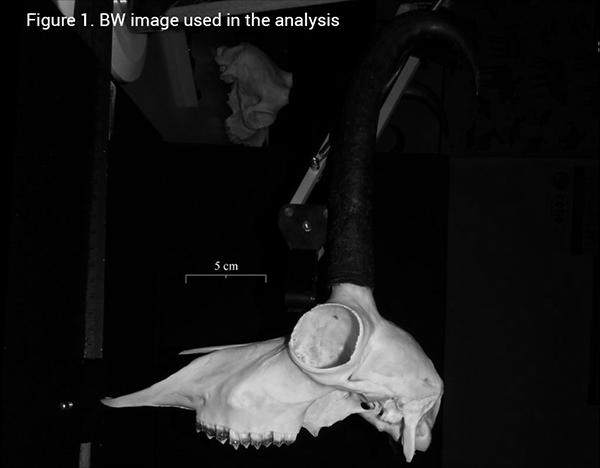
plt.imshow(gwashBW, 'gray') #this is matplotlib solution (Figure 1)
plt.xticks([]), plt.yticks([])
plt.show()

cv2.imshow('gwash', gwashBW) #this is for native openCV display
cv2.waitKey(0)

This image is suitable for automated online extraction of the skull, since there is a significant ammount of contrast of the object and the background. The idea is to use thresholding and a bit of erosion around the edges to delimit the skull from the rest of the picture and then apply automated contour extractions.

1
2
3
4
5
6
7
8
9
10
11
12
13
14
15
16

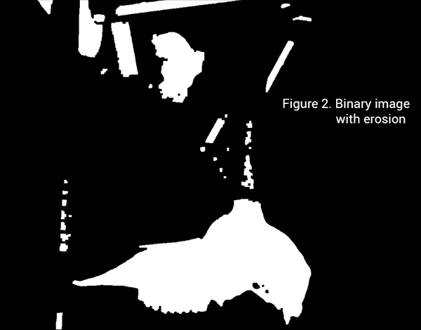
ret,thresh1 = cv2.threshold(gwashBW,15,255,cv2.THRESH_BINARY) #the value of 15 is chosen by trial-and-error to produce the best outline of the skull
kernel = np.ones((5,5),np.uint8) #square image kernel used for erosion
erosion = cv2.erode(thresh1, kernel,iterations = 1) #refines all edges in the binary image

opening = cv2.morphologyEx(erosion, cv2.MORPH_OPEN, kernel)
closing = cv2.morphologyEx(opening, cv2.MORPH_CLOSE, kernel) #this is for further removing small noises and holes in the image

plt.imshow(closing, 'gray') #Figure 2
plt.xticks([]), plt.yticks([])
plt.show()

contours, hierarchy = cv2.findContours(closing,cv2.RETR_TREE,cv2.CHAIN_APPROX_SIMPLE) #find contours with simple approximation

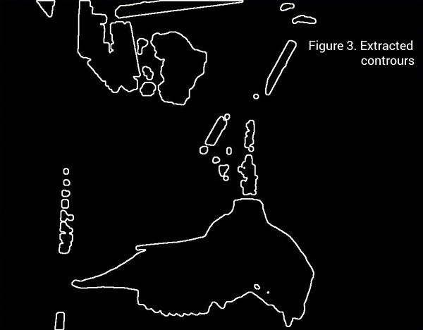
cv2.imshow('cleaner', closing) #Figure 3
cv2.drawContours(closing, contours, -1, (255, 255, 255), 4)
cv2.waitKey(0)

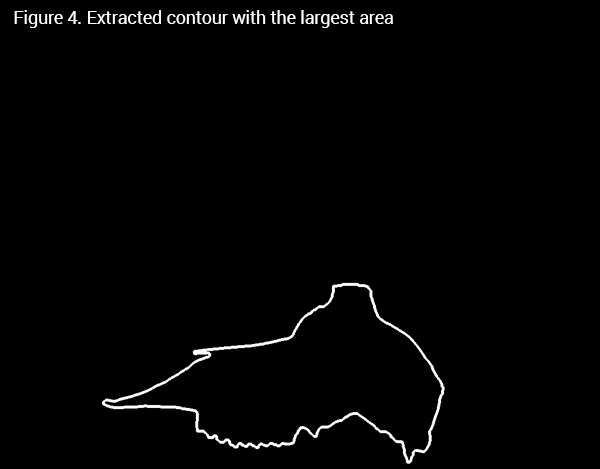
Finally, since other objects of no interest are also outlined in Figure 3, the skull outline must be identified in the array list contours. This can be done by a for loop, and the openCV method for calculating outline areas, as the skull outline is the longest continual outline in the image.

1
2
3
4
5
6
7
8
9
10
11
12
13
14
15

areas = [] #list to hold all areas

for contour in contours:
  ar = cv2.contourArea(contour)
  areas.append(ar)

max_area = max(areas)
max_area_index = areas.index(max_area) #index of the list element with largest area

cnt = contours[max_area_index] #largest area contour

cv2.drawContours(closing, [cnt], 0, (255, 255, 255), 3, maxLevel = 0)
cv2.imshow('cleaner', closing)
cv2.waitKey(0)
cv2.destroyAllWindows()

The extracted contour is a numpy array with xy coordinates of contour points in rows, so it can be directly used for sampling landmarks along the outline for fitting the normalized Fourier transform and doing shape analysis further. Of course, the procedure can be easily generalized to work over all images in a dataset, extract the contours with largest areas from each image, and generate a dataset for shape analysis.